If we consider the Mexican Hat potential discussed in the previous blog post, as a stand in for a soft phonon mode, a fundamental question in chemical physics is how regularly the mode tunnels between the vibrational states localised on one side, versus the other.
Classically, the chance of crossing over is zero, unless you have sufficient energy to overtop the barrier. From a Statistical Physics point of view, at finite temperature, some states will be Boltzmann populated with sufficient energy, and from this fraction and an attempt frequency from the rate of oscillation within an individual well, you could approximate the classical rate. You could directly extract this rate from a Molecular Dynamics simulation, including anharmonic and correlation terms, but even with ab-initio molecular dynamics, your nuclear coordinate is classical.
However, there is, of course, also quantum mechanical tunnelling directly through the barrier. The boss (@lonepair) asked me to consider whether this rate was easily calculable, to complement the considerable soft-phonon work occurring in the group.
To calculate this rate, there are a number of different approaches you could
take.
This includes semi-classical WKB theory, and methods used in small polaron hopping.
Here I start with a very general analytic quantum mechanical analysis, which
seems to to give you a very nice and general result to then use with your
numeric method.
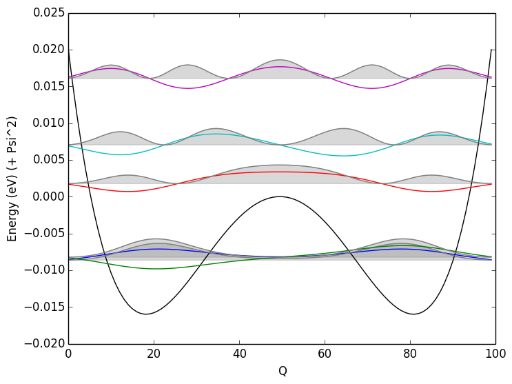
Mexican Hat confined modes
If we look at the states (\(\Psi_n\)) localised in the wells, you can see that the first state is symmetric, and the then the second state is anti-symmetric. The Pauli exclusion principle leads to a slight splitting in the degeneracy.
Our Hamiltonian is time independent, which means that we can use our eigenstates as a basis $$\Psi_n(Q,t) = \Psi_n(Q).e^{-i \omega_n t}$$
As expected, the time-dependence of this wavefunction just leads to a phase term (entirely imaginary dependence on \(t\)), as the \(\Psi_n\) are eigenstates of a time-independent Hamiltonian. The states will just beat at a characteristic frequency.
So let’s construct a wavepacket of \(\Psi_1\) and \(\Psi_2\).
$$\Phi(Q,t)=\frac{1}{\sqrt{2}} \left( \Psi_1(Q,t) + \Psi_2(Q,t) \right)$$
Expand to our time-dependent form above,
$$\Phi(Q,t)=\frac{1}{\sqrt{2}} \left( \Psi_1(Q).e^{-i \omega_1 t} + \Psi_2(Q).e^{-i \omega_2 t} \right)$$
Bring out the base frequency-beating term,
$$\Phi(Q,t)=\frac{1}{\sqrt{2}} e^{-i \omega_1 t} \left( \Psi_1(Q) + \Psi_2(Q).e^{-i (\omega_2-\omega_1) t} \right)$$
The observable we are interested in is the location of the wavepacket. We evaluate the probability density function by calculating the state’s expectation value with the position operator
Not 100% sure I got all the algebra correct there :^) But the key thing is that the state is phasing between
$$ \lvert\Psi_1\rangle \;\rightarrow\; \lvert\Psi_1\Psi_2\rangle \;\rightarrow\; \lvert\Psi_2\rangle \;\rightarrow\; \lvert\Psi_2\Psi_1\rangle \;\circlearrowright$$
The \(\Psi_1\) and \(\Psi_2\) states are de-localised between the two wells, but as these are Even and Odd wavefunctions, the combinations will be localised in state 1 and state 2.
And there’s only one, obvious, time constant generated by the phase term
$$e^{-i (\omega_2-\omega_1) t}$$
By Euler’s identity, \(e^{i\pi}=-1\)
$$\tau=(\omega_2-\omega_1)/\pi$$
By \(E=\hbar\omega , \omega=E/\hbar\), this is
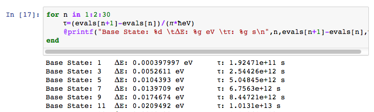
$$\tau = \frac{E_2-E_1}{\pi\hbar}$$
So really quite trivial! The time constant of beating between the states (tunnelling through the potential barrier) is directly related to the degeneracy splitting of the states. This makes sense as in the semi-classical picture, the degeneracy splitting is linked to the magnitude of the transfer (wavefunction overlap) integral between state 1 and 2.
I was initially concerned that there was no mass term here—obviously mass should come into the time constant of tunnelling! But it is there, hidden in the solution of the Time Independent Schrödinger Equation.
For the potential + states above, the values are not so ridiculous
Time to tunnel between states
Classically, with a harmonic potential, you would have a Simple Harmonic Oscillator with
$$\tau=\frac{2\pi}{\omega}$$
where
$$\omega=\sqrt{\frac{k}{m}}$$
For this system at a finite temperature, we should be able to consider a Bose-Einstein distribution of weights, and then collect an overall tunnelling time constant by summing the weighted rates. I haven’t yet tried this.
$$\tau_{total} = \left( \frac{p_1}{\tau_1} + \frac{p_2}{\tau_2} + \frac{p_3}{\tau_3} … \right)^{-1} $$
It was very enjoyable to find myself doing some basic pen + paper physics!